Fundamentals of Differential Equations Continuous Unique Solutions

Although there are methods for solving many differential equations, it is impossible to find useful formulas for the solutions of all of them. Whether we are looking for exact solutions or numerical approximations, it is useful to know conditions that imply the existence and uniqueness of solutions of initial value problems. In this section we state such a condition and illustrate it with examples.

Caution

If you have not had Math 402 (multivariable calculus), then you will need to read Appendices 11.1 and 11.2 before continuing.

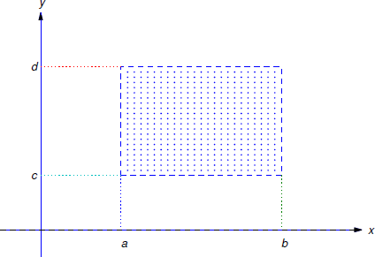
Some terminology: an open rectangle \(R\) is a set of points \((x,y)\) such that

\[ a < x < b \quad \text{and} \quad c < y < d \nonumber\]

(Figure 1.2.1 ). We'll denote this set by \(R: \{ a < x < b, c < y < d \}\). "Open" means that the boundary rectangle (indicated by the dashed lines in Figure 1.2.1 ) is not included in \(R\).

Figure 1.2.1 : An open rectangle

The next theorem gives sufficient conditions for existence and uniqueness of solutions of initial value problems for first order differential equations. We omit the proof, which is beyond the scope of this book.

Theorem 1.2.1 : Existence and Uniqueness

1. If \(f\) is continuous on an open rectangle \[R: \{ a < x < b, c < y < d \} \nonumber\] that contains \((x_0,y_0)\) then the initial value problem \[\label{eq:2.3.1} y'=f(x,y), \quad y(x_0)=y_0\] has at least one solution on some open subinterval of \((a,b)\) that contains \(x_0.\)
2. If both \(f\) and \(f_y\) are continuous on \(R\) then Equation \ref{eq:2.3.1} has a unique solution on some open subinterval of \((a,b)\) that contains \(x_0\).

It's important to understand exactly what Theorem 1.2.1 says.

• (a) is an existence theorem . It guarantees that a solution exists on some open interval that contains \(x_0\), but provides no information on how to find the solution, or to determine the open interval on which it exists. Moreover, (a) provides no information on the number of solutions that Equation \ref{eq:2.3.1} may have. It leaves open the possibility that Equation \ref{eq:2.3.1} may have two or more solutions that differ for values of \(x\) arbitrarily close to \(x_0\). We will see in Example 1.2.6 that this can happen.
• (b) is a uniqueness theorem . It guarantees that Equation \ref{eq:2.3.1} has a unique solution on some open interval \((a,b)\) that contains \(x_0\). However, if \((a,b)\ne(-\infty,\infty)\), Equation \ref{eq:2.3.1} may have more than one solution on a larger interval that contains \((a,b)\). For example, it may happen that \(b<\infty\) and all solutions have the same values on \((a,b)\), but two solutions \(y_1\) and \(y_2\) are defined on some interval \((a,b_1)\) with \(b_1>b\), and have different values for \(b<x<b_1\); thus, the graphs of \(y_1\) and \(y_2\) "branch off" in different directions at \(x=b\). (See Example 1.2.7 and Figure 1.2.3 ). In this case, continuity implies that \(y_{1}(b) = y_{2}(b)=\overline{y}\) (call their common value \(y\)), and \(y_{1}\) and \(y_{2}\) are both solutions of the initial value problem

\[\label{eq:2.3.2}y=f(x,y),\quad y(b)=\overline{y}\]

that differ on every open interval that contains \(b\). Therefore \(f\) or \(f_y\) must have a discontinuity at some point in each open rectangle that contains \((b, y)\), since if this were not so, \ref{eq:2.3.2} would have a unique solution on some open interval that contains \(b\). We leave it to you to give a similar analysis of the case where \(a > −∞\).

Example 1.2.1

Consider the initial value problem

\[\label{eq:2.3.3} y'={x^2-y^2 \over 1+x^2+y^2}, \quad y(x_0)=y_0.\]

Since

\[f(x,y) = {x^2-y^2 \over 1+x^2+y^2} \quad \text{and} \quad f_y(x,y) = -{2y(1+2x^2)\over (1+x^2+y^2)^2} \nonumber\]

are continuous for all \((x,y)\), Theorem 1.2.1 implies that if \((x_0,y_0)\) is arbitrary, then Equation \ref{eq:2.3.3} has a unique solution on some open interval that contains \(x_0\).

Example 1.2.2

Consider the initial value problem

\[\label{eq:2.3.4} y'={x^2-y^2 \over x^2+y^2}, \quad y(x_0)=y_0.\]

Here

\[f(x,y) = {x^2-y^2 \over x^2+y^2}\quad \text{and} \quad f_y(x,y) = -{4x^2y \over (x^2+y^2)^2} \nonumber\]

are continuous everywhere except at \((0,0)\). If \((x_0,y_0) \ne(0,0)\), there's an open rectangle \(R\) that contains \((x_0,y_0)\) that does not contain \((0,0)\). Since \(f\) and \(f_y\) are continuous on \(R\), Theorem 1.2.1 implies that if \((x_0,y_0)\ne(0,0)\) then Equation \ref{eq:2.3.4} has a unique solution on some open interval that contains \(x_0\).

Example 1.2.3

Consider the initial value problem

\[\label{eq:2.3.5} y'={x+y\over x-y},\quad y(x_0)=y_0.\]

Here

\[f(x,y) = {x+y\over x-y}\quad \text{and} \quad f_y(x,y) = {2x\over (x-y)^2} \nonumber\]

are continuous everywhere except on the line \(y=x\). If \(y_0\ne x_0\), there's an open rectangle \(R\) that contains \((x_0,y_0)\) that does not intersect the line \(y=x\). Since \(f\) and \(f_y\) are continuous on \(R\), Theorem 1.2.1 implies that if \(y_0\ne x_0\), Equation \ref{eq:2.3.5} has a unique solution on some open interval that contains \(x_0\).

Example 1.2.4

We will see later that the solutions of

\[\label{eq:2.3.6} y'=2xy^2\]

are

\[y\equiv0\quad \text{and} \quad y=-{1 \over x^2+c}, \nonumber\]

where \(c\) is an arbitrary constant. In particular, this implies that no solution of Equation \ref{eq:2.3.6} other than \(y\equiv0\) can equal zero for any value of \(x\). Show that Theorem \(\PageIndex{1b}\) implies this.

We'll obtain a contradiction by assuming that Equation \ref{eq:2.3.6} has a solution \(y_1\) that equals zero for some value of \(x\), but is not identically zero. If \(y_1\) has this property, there's a point \(x_0\) such that \(y_1(x_0)=0\), but \(y_1(x)\ne0\) for some value of \(x\) in every open interval that contains \(x_0\). This means that the initial value problem

\[\label{eq:2.3.7} y'=2xy^2,\quad y(x_0)=0\]

has two solutions \(y\equiv0\) and \(y=y_1\) that differ for some value of \(x\) on every open interval that contains \(x_0\). This contradicts Theorem 1.2.1 (b), since in Equation \ref{eq:2.3.6} the functions

\[f(x,y)=2xy^2 \quad \text{and} \quad f_y(x,y)= 4xy. \nonumber\]

are both continuous for all \((x,y)\), which implies that Equation \ref{eq:2.3.7} has a unique solution on some open interval that contains \(x_0\).

Note: \(y\equiv0\) is a singular solution since it cannot be obtained from the family \(y=-{1 \over x^2+c}, \nonumber\) by varying the parameter c.

Example 1.2.5

Consider the initial value problem

\[\label{eq:2.3.8} y' = {10\over 3}xy^{2/5}, \quad y(x_0) = y_0.\]

1. For what points \((x_0,y_0)\) does Theorem \(\PageIndex{1a}\) imply that Equation \ref{eq:2.3.8} has a solution?
2. For what points \((x_0,y_0)\) does Theorem \(\PageIndex{1b}\) imply that Equation \ref{eq:2.3.8} has a unique solution on some open interval that contains \(x_0\)?

Solution a

Since

\[f(x,y) = {10\over 3}xy^{2/5} \nonumber\]

is continuous for all \((x,y)\), Theorem 1.2.1 implies that Equation \ref{eq:2.3.8} has a solution for every \((x_0,y_0)\).

Solution b

Here

\[f_y(x,y) = {4 \over 3}xy^{-3/5} \nonumber\]

is continuous for all \((x,y)\) with \(y\ne 0\). Therefore, if \(y_0\ne0\) there's an open rectangle on which both \(f\) and \(f_y\) are continuous, and Theorem 1.2.1 implies that Equation \ref{eq:2.3.8} has a unique solution on some open interval that contains \(x_0\).

If \(y=0\) then \(f_y(x,y)\) is undefined, and therefore discontinuous; hence, Theorem 1.2.1 does not apply to Equation \ref{eq:2.3.8} if \(y_0=0\).

Example 1.2.6

Example 1.2.5 leaves open the possibility that the initial value problem

\[\label{eq:2.3.9} y'={10 \over 3}xy^{2/5}, \quad y(0)=0\]

has more than one solution on every open interval that contains \(x_0=0\). Show that this is true.

Solution

By inspection, \(y\equiv0\) is a solution of the differential equation

\[\label{eq:2.3.10} y'={10 \over 3} xy ^{2/5}.\]

Since \(y\equiv0\) satisfies the initial condition \(y(0)=0\), it is a solution of Equation \ref{eq:2.3.9}.

Now suppose \(y\) is a solution of Equation \ref{eq:2.3.10} that is not identically zero. We will see in chapter 2 that we can obtain the family of solutions

\[\label{eq:2.3.11} y = (x^2+c)^{5/3}. \]

Applying our initial condition gives us a particular solution

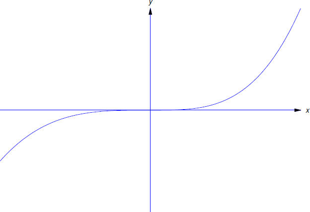
\[y=x^{10/3} \nonumber\]

as a second solution of Equation \ref{eq:2.3.9}. Both solutions are defined on \((-\infty,\infty)\), and they differ on every open interval that contains \(x_0=0\) (Figure 1.2.2 ).

Note: \(y\equiv0\) is a singular solution since it cannot be obtained from the family by varying c.

Figure 1.2.2 : Two solutions (\(y\equiv0\) and \(y=x^{10/3}\)) of Equation \ref{eq:2.3.9} that differ on every interval containing \(x_{0}=0\)

Example 1.2.7

From Example 1.2.5 , the initial value problem

\[\label{eq:2.3.12} y'={10 \over 3}xy^{2/5}, \quad y(0)=-1\]

has a unique solution on some open interval that contains \(x_0=0\). Find a solution and determine the largest open interval \((a,b)\) on which it is unique.

Solution

Let \(y\) be any solution of Equation \ref{eq:2.3.12}. Because of the initial condition \(y(0)=-1\) and the continuity of \(y\), there's an open interval \(I\) that contains \(x_0=0\) on which \(y\) has no zeros, and is consequently of the form Equation \ref{eq:2.3.11}. Setting \(x=0\) and \(y=-1\) in Equation \ref{eq:2.3.11} yields \(c=-1\), so

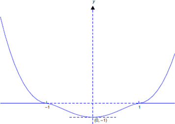
\[\label{eq:2.3.13} y=(x^2-1)^{5/3}\]

for \(x\) in \(I\). Therefore every solution of Equation \ref{eq:2.3.12} differs from zero and is given by Equation \ref{eq:2.3.13} on \((-1,1)\); that is, Equation \ref{eq:2.3.13} is the unique solution of Equation \ref{eq:2.3.12} on \((-1,1)\). This is the largest open interval on which Equation \ref{eq:2.3.12} has a unique solution. To see this, note that Equation \ref{eq:2.3.13} is a solution of Equation \ref{eq:2.3.12} on \((-\infty,\infty)\), but the solution below is another solution of Equation \ref{eq:2.3.12} that differs from Equation \ref{eq:2.3.13} on every open interval larger than \((-1,1)\):

\[y = \left\{ \begin{array}{cl} (x^2-1)^{5/3}, & -1 \le x \le 1, \\[6pt] 0, & |x|>1. \end{array} \right. \nonumber\]

Figure 1.2.3 : Two solutions of Equation \ref{eq:2.3.12} on (−1,1) that coincide on (−1, 1), but on no larger open interval.

Example 1.2.8

From Example 1.2.5 , the initial value problem

\[\label{eq:2.3.14} y'={10 \over 3}xy^{2/5}, \quad y(0)=1\]

has a unique solution on some open interval that contains \(x_0=0\). Find the solution and determine the largest open interval on which it is unique.

Solution

Let \(y\) be any solution of Equation \ref{eq:2.3.14}. Because of the initial condition \(y(0)=1\) and the continuity of \(y\), there's an open interval \(I\) that contains \(x_0=0\) on which \(y\) has no zeros, and is consequently of the form Equation \ref{eq:2.3.11}. Setting \(x=0\) and \(y=1\) in Equation \ref{eq:2.3.11} yields \(c=1\), so

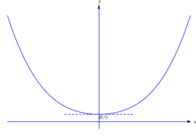
\[\label{eq:2.3.15} y=(x^2+1)^{5/3}\]

for \(x\) in \(I\). Therefore every solution of Equation \ref{eq:2.3.14} differs from zero and is given by Equation \ref{eq:2.3.15} on \((-\infty,\infty)\); that is, Equation \ref{eq:2.3.15} is the unique solution of Equation \ref{eq:2.3.14} on \((-\infty,\infty)\). Figure 1.2.4 ) shows the graph of this solution.

Figure 1.2.4 : The unique solution of Equation \ref{eq:2.3.14}.

mirandadelver.blogspot.com

Source: https://math.libretexts.org/Courses/Cosumnes_College/Math_420:_Differential_Equations_%28Breitenbach%29/01:_Introduction/1.02:_Existence_and_Uniqueness_of_Solutions

Share this post